Install SimTracker and run a parallel ring network simulation

There are three ways to install SimTracker: 1) using Docker, a virtual software container which has a preconfigured software environment that includes all software necessary to run SimTracker and NEURON in Linux or Mac, 2) by installing SimTracker on a system that has MATLAB, NEURON, and Mercurial or Git, and 3) by installing a stand-alone version of SimTracker that doesn’t require a separate MATLAB license on a system with NEURON and Mercurial/Git. The latter two options are available for Linux, Mac OS X, and Windows computers. In this tutorial, the user will use the first approach on a Linux computer to create a fresh instance of a Docker container with SimTracker installed. For other approaches, see our documentation at readthedocs.org <readthedocs.org>

1. To create a fresh container instance with SimTracker installed, install Docker either by downloading it from https://www.docker.com or by using the package manager corresponding to the Linux distribution on the computer. Docker installation instruction for different Linux distributions are available at https://docs.docker.com/engine/installation/linux/.

2. After installing Docker, download and install the SimTracker ringdemo image with the following command:

   terminal-$ docker pull solteszlab/simtracker

   This will download the SimTracker Docker image and save it on the computer.

3. Next, create a ‘repos’ directory which will be used for storing model code and results data generated when running simulations:

   terminal-$ mkdir repos

4. Then, start the SimTracker container by entering the following command:

   terminal-$ docker run --rm -it -e DISPLAY=$DISPLAY -v /tmp/.X11-unix:/tmp/.X11-unix -v $PWD/repos:/home/docker/repos solteszlab/simtracker

   Note: The options -e and -v ensure that GUI applications based on the X11 standard can run in the Docker container and their graphics can appear on the host computer. The second -v option mounts the newly created ‘repos’ directory as a volume inside the Docker container. It is important to mount this directory from the host computer, making it available within Docker. Unless special steps are taken, files and data saved to other directories within the Docker package, which are not accessible outside of Docker, will also not be available even within Docker after closing and reopening the Docker package.

5. Finally, run SimTracker with the following command:

   terminal-$ ./simtracker/run_SimTracker.sh

   SimTracker will start and ask for a repository directory. Select the ’ringdemo’ repository included in the sample repo directory within Docker.

6. To design a new simulation, from the Runs menu choose “Design Run”. The property fields in the SimTracker will become editable.

   

   Design new run menu item.

7. Enter a unique name for the simulation (allowed characters include letters, numbers, and the underscore character), such as MyFirstRingDemo.

   

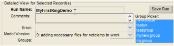
   Edit run name.

8. Optionally, enter comments about the simulation. It is often helpful to users if they note the specific question or idea that triggered them to run this particular simulation.

9. Specify the model code version to use for this simulation. Usually, this will be the most recent version of the code. The list of available code versions will correspond to each time users “committed” a version of the code in their model code repository and will also list the comments they entered when committing that code version. Select the most recent version, #9.

   

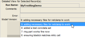
   Specify model code version.

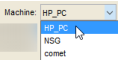
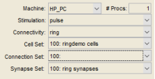
10. Specify the machine to use for running the simulation. For users to run this simulation on their own computers, they must find the unique name of their computer from the list and select it. Then, in the field to the right of the machine name, specify the number of processors to be used to execute the run. On a personal computer, users can either set this to 1 or, to run the network in parallel, set it to the total number of cores (aka processors) on their machines.

    

11. The default values in the various menus for simulation control (stimulation, connectivity algorithm, cell numbers, connection numbers, and synapse kinetics) can be used to run a ringdemo network of size XXXX (specify network configuration details that will be used).

    

12. Upon finishing the specification of simulation properties, click the “Save Run” button that appeared when upon starting to design the simulation. The simulation will now appear in the list of simulations at the top of the SimTracker. The property fields will become uneditable (to change the run prior to execution, choose “Edit Run” from the “Runs” menu). The process for executing a simulation differs somewhat depending on whether users are executing it on their personal computers, using the NSG portal, or accessing a supercomputer independently of the NSG portal. The following list details the process for using a personal computer. For instructions on using the NSG portal or a supercomputer directly, see Tutorial Design, execute and upload a simulation.

    

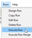
13. To execute the simulation, select its row from the table at the top of the SimTracker, and then from the “Runs” menu choose “Execute Run”.

    

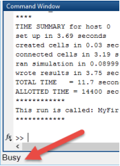
14. The computer”s CPU may become very active and users who are using MATLAB scripts to run the SimTracker, will see the MATLAB status bar display “Busy” until the simulation completes Additionally, a NEURON window may pop up.

    
    

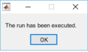
15. When the simulation finishes, a dialog box will appear that states “The run has been executed”. Once this message appears, continue to the next step.

    

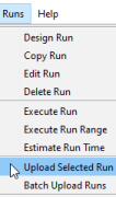
16. Select the simulation in the SimTracker (make sure to view the “Not Ran” view) and, from the “Runs” menu, choose “Upload Run” to display the results of the run in the SimTracker.

    

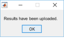
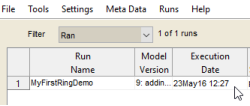
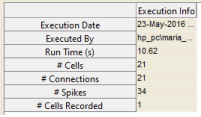
17. Once the simulation is successfully uploaded to the SimTracker, a dialog box will appear stating that “Results have been uploaded.” The SimTracker table will switch to the “Ran” view. In both the list of runs and the form view below, SimTracker will show the executed simulation”s run time, number of spikes, and execution date.

    
    
    

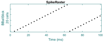
    After the simulation has been executed and uploaded, it is time to analyze the results. The ringdemo simulation produces a spikeraster file that contains the times found in Table [tab:outputs:raster], which compare well to the results from [HC08], found in section 3.3.5 Reporting simulation results.

18. Select the completed simulation of interest from the table in the SimTracker.

19. Look at the table on the bottom right side of the SimTracker for a list of available outputs for that particular simulation (the list will vary depending on which output files users choose to print for their simulations). For now, click to select the checkboxes next to the ‘Spike Raster’ and ‘Membrane Potential’ outputs.

    

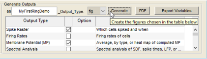
    Note: For more information on any particular output, click on that row to highlight that output type and then hover the mouse anywhere over the output table to see a tooltip with guidance about the selected output type.

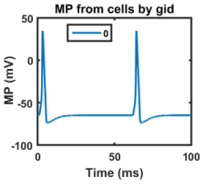
20. After selecting the outputs of interest, click the “Generate” button to produce them as MATLAB figures. If prompted to enter a GID (global ID number for a cell type), enter ‘0’ to display the membrane potential for cell #0. Users can zoom in, pan, and otherwise edit or save the figures once the MATLAB figures are generated.

    
    

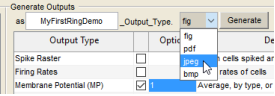
21. Alternatively, users can directly export the figures to an image format of their choice by selecting the “fig” menu option in the file extension pop-up menu and choosing a different file format (such as jpeg, bmp, pdf, etc.).

    

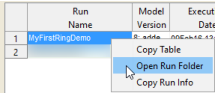
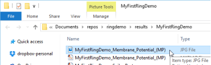
22. Exported images will be saved in the results folder for that particular simulation, which will be logged in the figure-generation log on the lower left side of the SimTracker. To view the file location of the saved image, users can right click in the figure-generation log or in the main simulation list window and choose to open the simulation results directory.

    
    

When done using SimTracker, the Docker container can be exited with the ‘exit’ command. Please consult the online Docker documentation at https://docs.docker.com/engine/userguide/containers/dockerimages/ for further details on how to use Docker images and software containers, including use of the ‘docker commit’ command to save data and settings within the package.

• Tutorials
• Create a new model repository using SimTracker
• Design, execute and upload a simulation
• Organize simulations
• Analyzing a simulation
• Network Clamp